Kimi Linear and KDA: From Channel-Wise Forgetting to Hardware-Efficient Linear Attention
Summary and core assessment
Kimi Linear does not merely ask how to approximate Softmax more cheaply. Its narrower and more useful question is how a fixed-size linear-attention state should forget selectively while remaining parallelizable on GPUs. Kimi Delta Attention (KDA) replaces Gated DeltaNet’s single decay coefficient with a channel vector, so each row of the state matrix can operate at a different time scale. It also restricts the update to a special diagonal-plus-low-rank (DPLR) form. That restriction removes secondary chunking and several matrix multiplications from the general algorithm. Kimi Linear then interleaves three KDA layers with one MLA layer: most layers use compressed, fixed-state memory, while a minority retain token-level retrieval.
The headline numbers refer to different experiments. The 1.4T-token models form the controlled architectural comparison. The released checkpoint was trained on 5.7T tokens. The 1M number is its maximum context window after long-context training. Efficiency also has three meanings: Figure 7 reports roughly 2.2x batch-one decoding TPOT at 1M; Figure 1 reports 6.3x TPOT when the smaller cache enables a larger batch; and “up to 75% KV-cache reduction” concerns memory capacity. Latency, batched throughput, and cache footprint are not interchangeable.
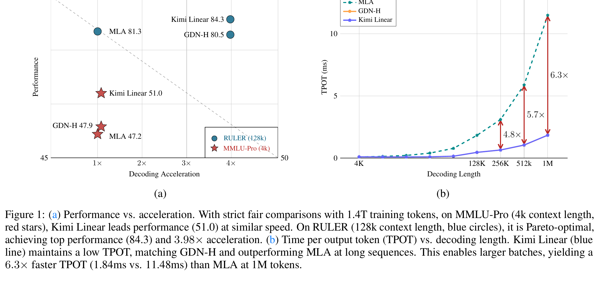
Source: Kimi Linear, Figure 1, page 1.
My assessment has five parts. First, KDA adds forgetting resolution, not unlimited memory capacity; a fixed matrix still compresses and interferes. Second, the 3:1 hybrid is not an embarrassed compromise. It uses a small number of MLA layers to repair a structural weakness of purely recurrent state: exact access to old tokens. Third, 1.16x scaling efficiency is a meaningful but restrained training result, not a sixfold training speedup. Fourth, the system gain depends on kernels, layer ratio, parallelism, and batching; the recurrence alone is insufficient to reproduce it. Fifth, FlashKDA, Gated DeltaNet-2, and Preconditioned DeltaNet expose three boundaries of the original design: the kernel can still improve, erase and write share one scalar gate, and the delta rule remains a first-order update that ignores regression curvature.
1. Evidence boundaries: three model regimes under one name
The paper’s main controlled experiment compares Kimi Linear, hybrid Gated DeltaNet (GDN-H), and MLA with matched architecture size, parameter count, and training setup. Each model receives 1.4T tokens. Figure 1, Table 5, and the reinforcement-learning comparison primarily belong to this regime. “84.3 on RULER,” “54.5 average long-context score,” and the RL curves are therefore claims about these matched 1.4T models, not universal properties of every KDA implementation.
The released Kimi-Linear-48B-A3B-Instruct is a separate regime. Its model card reports 5.7T pretraining tokens, 48B total parameters, about 3B active parameters, and a 1M context configuration. The first number is training volume and the second is a window limit. Neither invalidates the 1.4T ablations; controlled causal claims still come from the smaller matched setting. The released weights are useful for checking inference and implementation, but they cannot replace the paper’s controls.
The third regime is post-paper engineering. The official model initially relied on Flash Linear Attention (FLA), while Moonshot AI later released FlashKDA. FlashKDA changes chunk size, state precision, and kernel organization. It answers how much faster the same operator can run; it does not re-establish model quality. Multiplying its roughly 2x kernel speedup by a model-level TPOT number would be invalid because MoE, MLA layers, communication, scheduling, and memory traffic become new bottlenecks.
This note prioritizes the paper and official configuration for facts, and official FLA/FlashKDA code for execution paths. A Zhihu reading, Scientific Spaces’ history of linear attention, MZeroMiko’s derivation, and an affine-transform derivation help compare explanations only. Numerical and causal claims are checked against primary material. I did not reproduce the 1.4T training run, so public curves are reported as paper results rather than independent measurements.
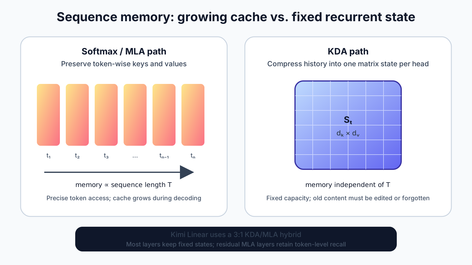
Based on Kimi Linear, Sections 3–4, and the released model configuration.
“Fixed” describes a state size that does not grow with sequence length; it does not mean lossless storage. Softmax preserves per-token keys and values and can revisit them. KDA compresses the past into one matrix per head, removing linearly growing decoding cache but forcing the model to decide online what to retain and overwrite. Memory management is the central modeling problem created by linear attention’s systems advantage.
2. From correlation accumulation to directed rewriting
Consider the simplest linear attention recurrence. Let \(q_t\in\mathbb{R}^{d_k}\), \(k_t\in\mathbb{R}^{d_k}\), \(v_t\in\mathbb{R}^{d_v}\), and \(S_t\in\mathbb{R}^{d_k\times d_v}\). Omitting feature-map notation gives:
\[ S_t = S_{t-1} + k_t v_t^{\top}, \qquad o_t = S_t^{\top} q_t. \]
Unrolling yields \(S_t=\sum_{i=1}^{t}k_iv_i^{\top}\). Every key–value association is added directly. Complexity is linear in sequence length and decoding state is fixed-size, but similar keys write into the same direction. A new association has no explicit way to replace the old one, so finite states accumulate interference.
DeltaNet introduces the Widrow–Hoff delta rule. It first predicts the value at the current key, \(\hat v_t=S_{t-1}^{\top}k_t\), and writes only the residual:
\[ S_t = S_{t-1} + \beta_t k_t\left(v_t-S_{t-1}^{\top}k_t\right)^{\top}. \]
Equivalently,
\[ S_t = \left(I-\beta_t k_tk_t^{\top}\right)S_{t-1} + \beta_t k_tv_t^{\top}. \]
\(\beta_t\) controls edit strength. The first term erases the old prediction in the present key direction; the second writes the new value. This is address-directed editing rather than blind accumulation. Old directions that are not selected by \(k_t\) can nevertheless persist. Gated DeltaNet therefore adds a scalar \(\alpha_t\) that lets the entire state forget:
\[ S_t = \alpha_t\left(I-\beta_t k_tk_t^{\top}\right)S_{t-1} + \beta_t k_tv_t^{\top}. \]
All key channels within a head share that clock. If some channels encode local syntax while others retain cross-section entities, they are still scaled together. KDA turns the scalar into \(\alpha_t\in(0,1)^{d_k}\) and applies it along the key dimension:
\[ S_t = \left(I-\beta_t k_tk_t^{\top}\right) \mathrm{Diag}(\alpha_t)S_{t-1} + \beta_t k_tv_t^{\top}, \qquad o_t=S_t^{\top}q_t. \]
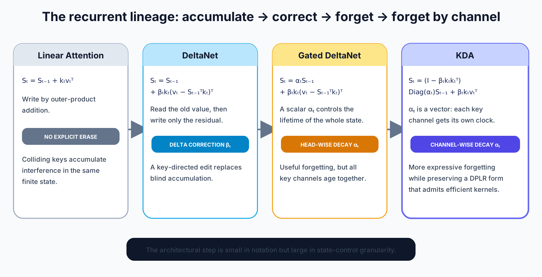
Equations follow Kimi Linear, Sections 2–3, and Gated DeltaNet.
The order matters: \(\mathrm{Diag}(\alpha_t)\) first decays the old state, \(I-\beta_tk_tk_t^{\top}\) then erases along the current key, and \(\beta_tk_tv_t^{\top}\) writes the new association. Because the decay multiplies on the left, it scales rows associated with key channels, not value-dimension columns. “One forget gate per neuron” is too vague; “one decay coefficient per key channel in each head” is precise.
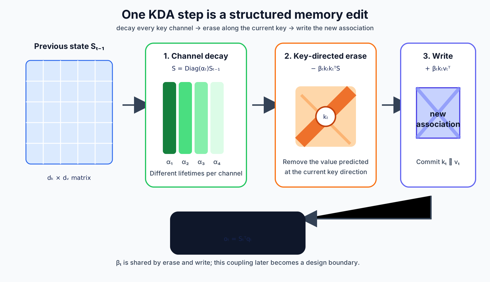
Based on Equation 10 of the paper.
“Decay–erase–write” is an explanatory decomposition, not three independent learned gates. KDA makes \(\alpha_t\) channel-wise, but \(\beta_t\) remains scalar and jointly controls erase and write. The original parameterization cannot directly express aggressive erasure with cautious writing. That coupling later motivates Gated DeltaNet-2.
3. From token-by-token recurrence to WY/UT chunk parallelism
The recurrence is ideal for decoding but poor for long-sequence training. A strict loop over \(t=1,2,\ldots,T\) exposes only tiny matrix operations, and each step waits for the previous state. Linear asymptotic complexity does not imply hardware efficiency; a serial \(O(T)\) algorithm may lose to highly parallel attention.
KDA belongs to the DPLR transition family:
\[ S_t = \left(D_t-a_tb_t^{\top}\right)S_{t-1}+u_tv_t^{\top}, \]
with the KDA identification
\[ D_t=\mathrm{Diag}(\alpha_t), \qquad a_t=\beta_tk_t, \qquad b_t=k_t\odot\alpha_t, \qquad u_t=\beta_tk_t. \]
The general DPLR algorithm combines repeated “diagonal minus rank-one” transforms within a chunk into a compact WY representation. Instead of explicitly materializing every product, it organizes accumulated diagonal factors and low-rank corrections as a triangular system, then computes an entire token block with GEMMs. UT is the corresponding transposed/upper-triangular organization used to map dependencies to efficient matrix products and triangular solves.
KDA’s constraint is the important part. In generic DPLR, \(D_t\), \(a_t\), and \(b_t\) are independent, so block products need smaller secondary chunks to control intermediates and dependencies. In KDA, \(b_t=k_t\odot\alpha_t\) shares structure with \(D_t\) and \(k_t\). The paper exploits this relation to remove two secondary-chunking stages and about three matrix multiplications. Recurrence is not eliminated; it becomes parallel within each chunk, with a compact state passed between chunks.
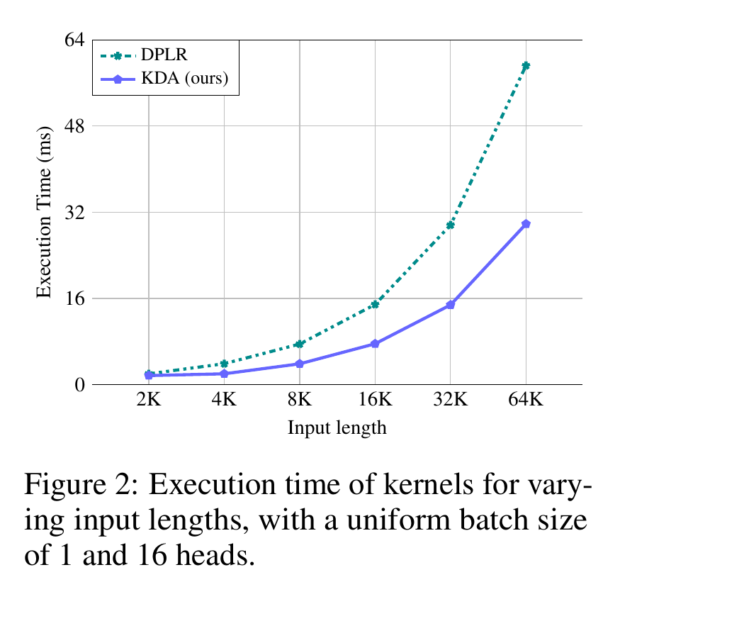
Source: Kimi Linear, Figure 2, page 5.
Figure 2 uses batch size one and 16 heads. At 64K, the KDA curve is roughly half the general DPLR time. This isolates a benefit from structured parameterization but does not imply a 2x speedup for a complete 48B MoE. Projections, convolution, normalization, gating, MoE, MLA layers, and communication remain.
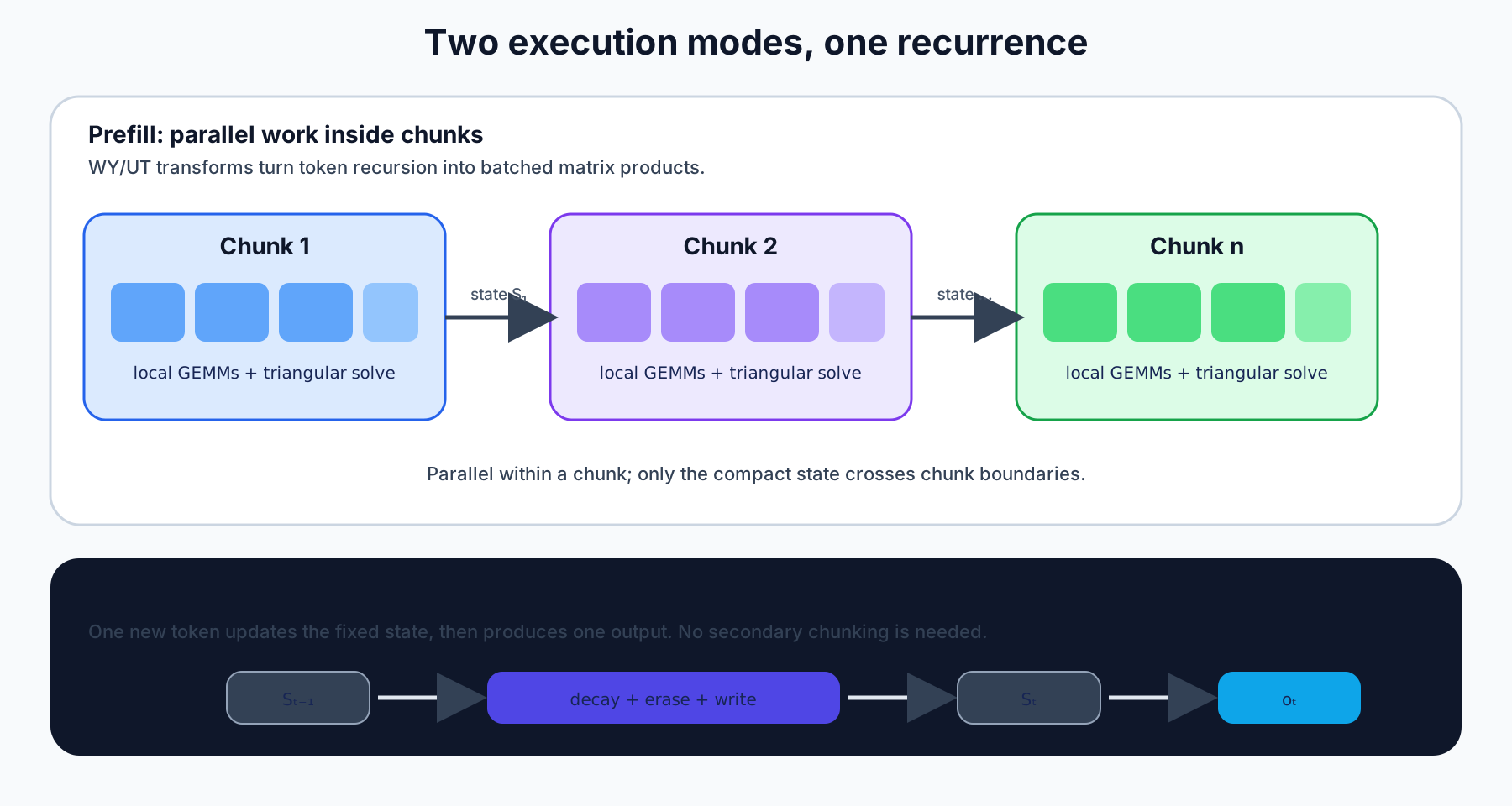
Based on Section 3.2, the paper’s appendix algorithms, and FLA’s KDA kernel paths.
Chunking also changes floating-point association. A low-precision chunk result need not be bit-identical to a token recurrence. Verification should compare outputs, final states, and gradients across long sequences, extreme decay values, and variable-length batches. FlashKDA’s later choice—BF16 state storage with FP32 FMA—explicitly trades memory bandwidth against accumulated error.
4. KDA is more than one recurrence: assembling the full block
The block projects the hidden state into \(q,k,v\). All three paths use ShortConv and Swish/SiLU, giving each token a small local receptive field before recurrence. Queries and keys receive L2 normalization so vector magnitude does not simultaneously act as address direction and write strength. A separate projection plus sigmoid produces \(\beta_t\). A low-rank decay projection first maps to a smaller dimension and then to per-head, per-key-channel decay, avoiding a costly direct \(H\times d_k\) gate projection.
Decay is parameterized in log space so \(\alpha_t\) stays in \((0,1)\) and can represent time scales close to one. Conceptually,
\[ g_t=-\exp(A)\odot\mathrm{softplus}(z_t+b), \qquad \alpha_t=\exp(g_t). \]
\(g_t\) is non-positive, so decay cannot amplify old state. FLA’s symbols and layouts can change across versions. Code readers should check whether a kernel receives log decay or exponentiated \(\alpha_t\) rather than inferring semantics from a variable name.
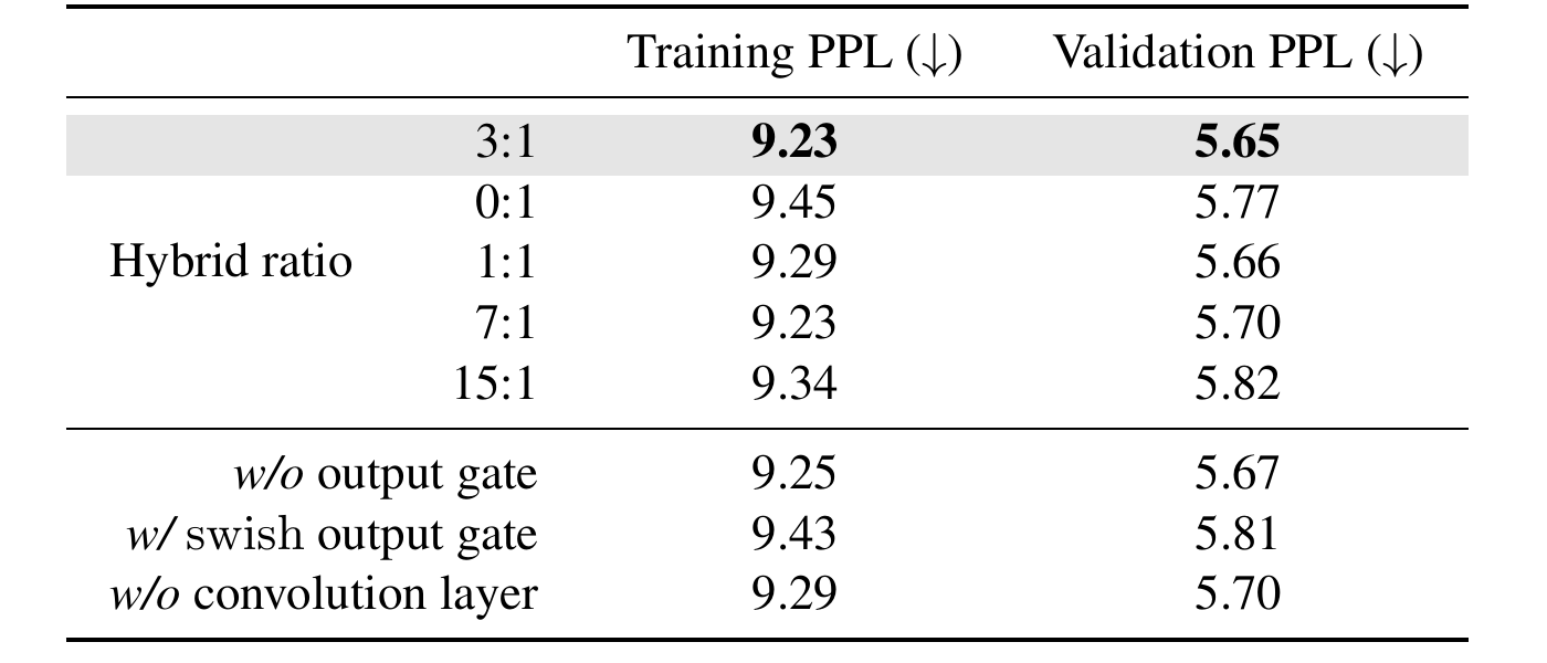
The recurrent output is head-wise RMS-normalized, multiplied by a sigmoid output gate, and projected back to model dimension. The output gate selects recurrent content for the residual stream; it is distinct from the memory-lifetime gate \(\alpha_t\) and the edit-strength gate \(\beta_t\). Removing it changes validation PPL from 5.65 to 5.67 in Table 1, while replacing it with a Swish gate yields 5.81. The gate form is not freely interchangeable in this setup.
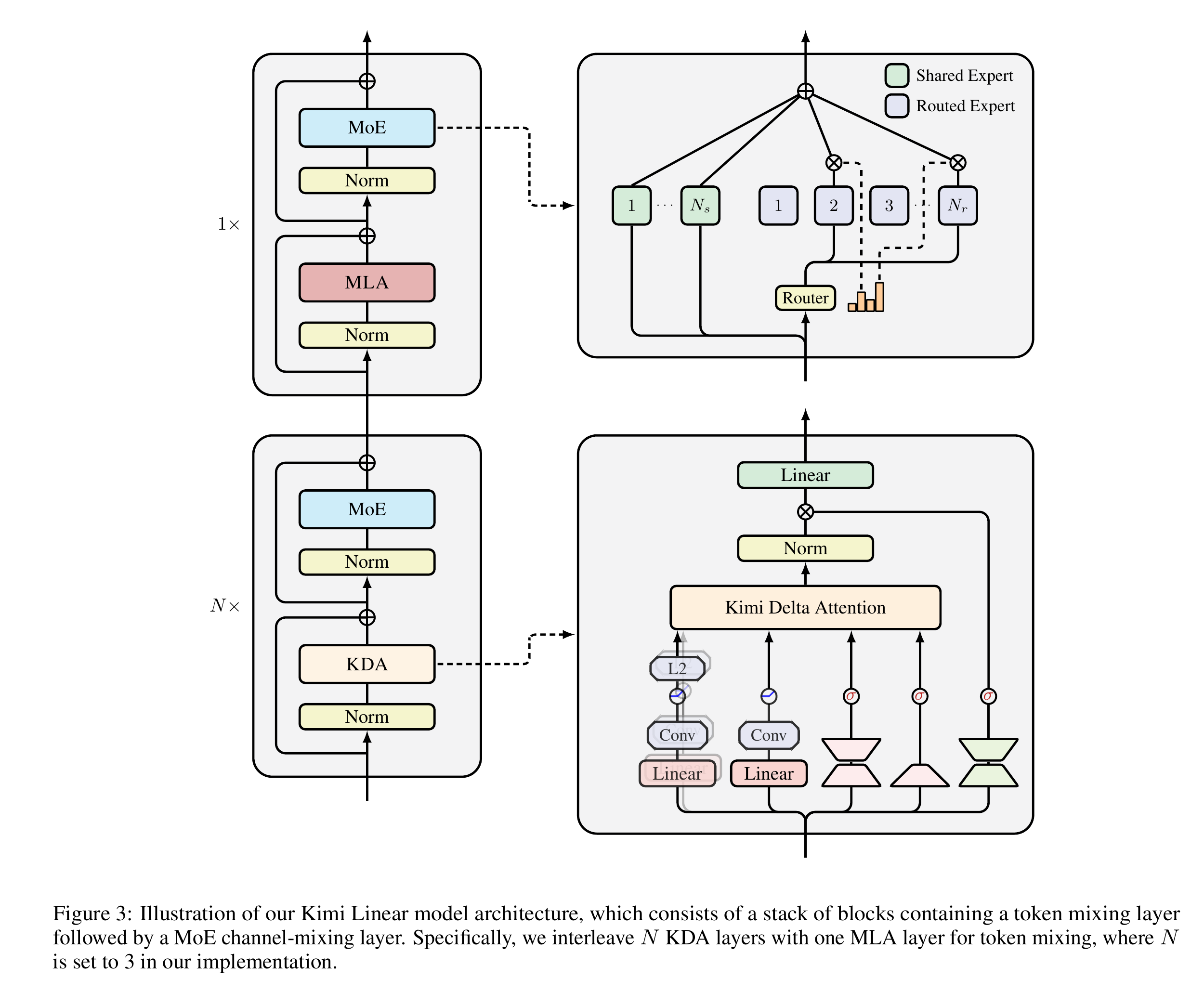
Source: Kimi Linear, Figure 3, page 6.
The released configuration contains 27 token mixers: 20 KDA layers at 1–3, 5–7, and so on, plus seven MLA layers at 4, 8, 12, 16, 20, 24, and 27. Because the final layer is MLA, the exact count is 20:7 rather than a literal integer 3:1. It also specifies hidden size 2304, 32 KDA heads of dimension 128, 256 routed experts with top-8 selection, and a shared expert. These are current checkpoint facts; details in the paper’s controlled 1.4T models are not identical.
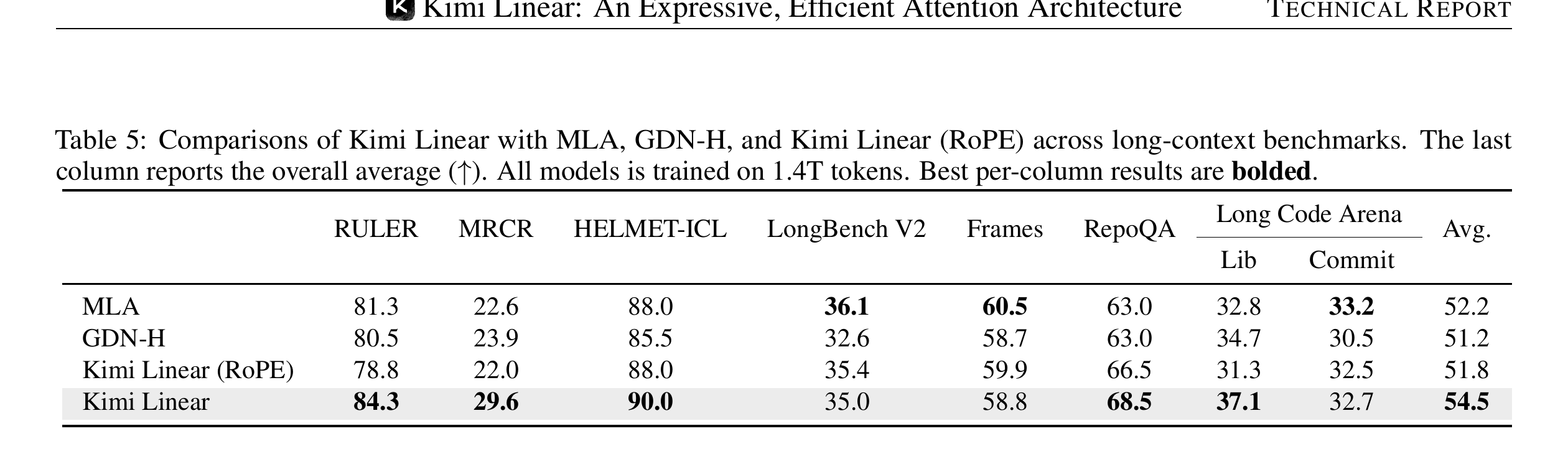
Kimi Linear uses NoPE. KDA recurrence already supplies causal order through state updates. For MLA, removing RoPE avoids frequency-base or YaRN-style retuning during context extension and enables a simpler MQA-style inference conversion. The cost is losing explicit relative-position rotation; hierarchy, local convolution, and content must learn distance. In Table 5, NoPE averages 54.5 versus 51.8 for the RoPE variant, but it does not win every column. The evidence does not establish that NoPE is generally superior to RoPE.
5. Experiment I: what the synthetic tasks establish
Palindrome, Multi-Query Associative Recall (MQAR), and stack tracking test exact copying, key–value recall, and state-machine updates. The paper trains two-layer, two-head models with head dimension 128 for at most 20K steps and searches a learning-rate grid. Top panels vary sequence length and report peak training accuracy; bottom panels fix length 1024 and compare convergence.
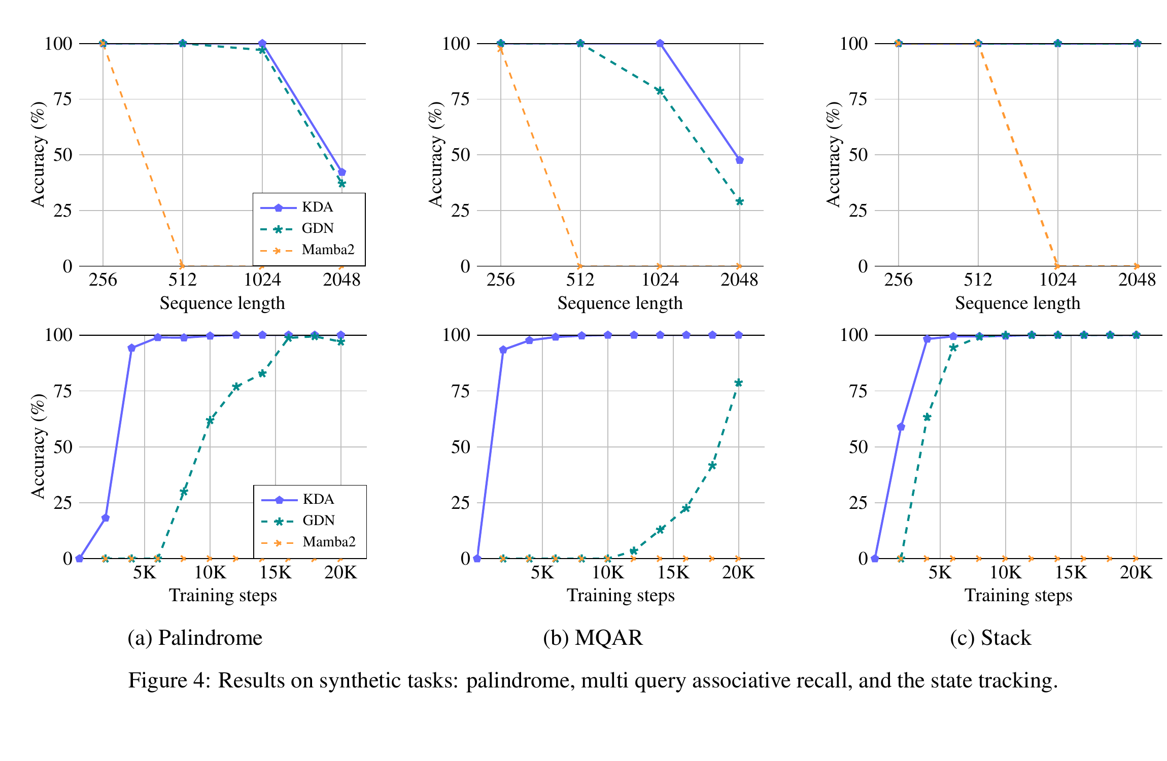
Source: Kimi Linear, Figure 4, page 7.
KDA reaches high accuracy faster than GDN on all three tasks. MQAR is especially clear: KDA approaches full accuracy around 5K steps, while GDN remains lower at 20K. At length 2048, KDA also exceeds GDN on palindrome and MQAR. This is consistent with the motivation that one head can assign different lifetimes to different address directions.
The experiment establishes easier learning in small controlled memory problems, not lossless storage of arbitrary long text. It also does not eliminate the possibility that the learning-rate grid favors architectures differently. Real language introduces aliases, noise, cross-document conflict, and ambiguous queries. Claiming that KDA “solves linear attention capacity” would exceed the evidence.
6. Experiment II: ablating the 3:1 ratio, convolution, and output gate
Table 1 jointly tests hybrid ratio and block components. MLA-only (0:1) reaches train/validation PPL 9.45/5.77; 1:1 reaches 9.29/5.66; 3:1 reaches 9.23/5.65; 7:1 matches 9.23 train PPL but worsens validation to 5.70; and 15:1 reaches 9.34/5.82. The result is not “more KDA is always better.” A minority of MLA layers remains important for generalization. The differences are small enough that the optimal ratio may move with data, scale, or kernel cost.
Source: Kimi Linear, Table 1, page 8.
Removing ShortConv yields 9.29/5.70, evidence that local mixing helps but not that convolution is the central source of quality. Removing the output gate yields 9.25/5.67; a Swish output gate is markedly worse at 9.43/5.81. A defensible conclusion is that the chosen sigmoid gate matches the surrounding normalization and residual scale. The table does not individually ablate Q/K L2Norm, low-rank decay projection, or NoPE, nor does it measure their isolated gains in the released model.
7. Experiment III: reading 1.16x scaling efficiency correctly
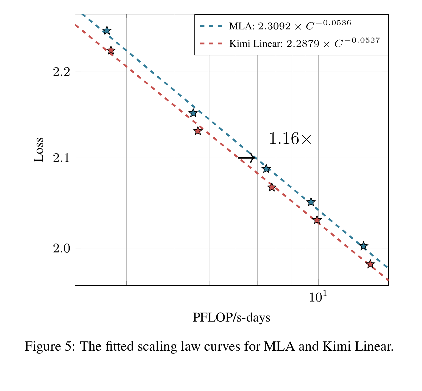
The paper fits loss–compute curves to MoE models from 653M to 1.7B active parameters. MLA fits \(2.3092C^{-0.0536}\) and Kimi Linear fits \(2.2879C^{-0.0527}\). Near equal target loss, their horizontal separation is about 1.16x, which the authors call computational efficiency.
Source: Kimi Linear, Figure 5, page 9.
This is fitted training compute required for equal loss, not wall-clock training speed and not inference throughput. The exponents are nearly equal and much of the gap is in the intercept; the observed range contains only five scales. The paper notes that KDA reused MLA-oriented tuning, so further tuning might move the curve, but that is a hypothesis rather than measured gain. I find the modest number more informative than an order-of-magnitude claim: it shows that the hybrid did not purchase efficiency with an obvious quality collapse, while keeping the advantage auditable.
8. Long context and RL: average leadership is not a clean sweep
All four Table 5 models use 1.4T training tokens and are evaluated at 128K context. Kimi Linear leads RULER, MRCR, HELMET-ICL, RepoQA, and Long Code Arena Lib, averaging 54.5; MLA averages 52.2, GDN-H 51.2, and Kimi Linear with RoPE 51.8. Counterexamples matter: MLA scores 36.1 versus 35.0 on LongBench V2, 60.5 versus 58.8 on Frames, and 33.2 versus 32.7 on Long Code Arena Commit.
Source: Kimi Linear, Table 5, page 12.
The accurate statement is that Kimi Linear has the best average in this suite and leads several retrieval and repository tasks, not that it universally beats full attention. RULER emphasizes controlled retrieval; Frames integrates distributed evidence; LongBench V2 mixes more task types. Token-level access retained by MLA can still be decisive for the latter cases.
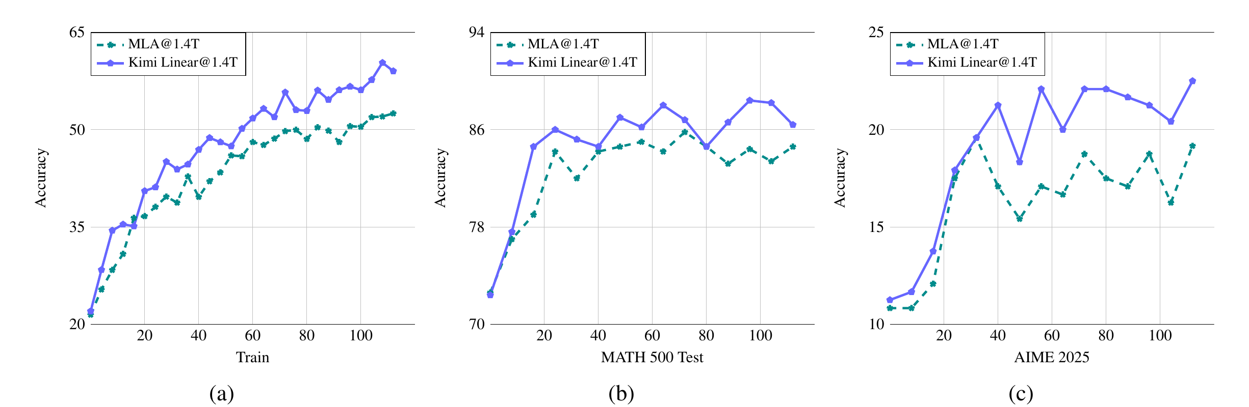
The paper also starts mathematical RL from matched 1.4T checkpoints. Initial MATH500 and AIME 2025 levels are similar, while Kimi Linear is mostly higher during training and evaluation. The curves support that the architecture survives and benefits from RL post-training, but do not identify why. Pretraining representation, recurrent inductive bias, sampling throughput, optimization noise, or hyperparameter interaction could contribute. One math-RL setup cannot establish that linear attention is generally better suited to RL.
Source: Kimi Linear, Figure 6, page 12.
9. Efficiency: separate single-request latency, batching, and cache
Figure 7 explicitly uses batch size one. At 512K, Kimi Linear is about 2.3x faster than MLA in prefill and 1.8x in TPOT; at 1M, the factors are about 2.9x and 2.2x. GDN-H and Kimi Linear are close, indicating that much of this systems gain comes from hybrid linear layers reducing long-sequence attention work. KDA’s modeling advantage over GDN does not automatically become an equal end-to-end latency advantage.
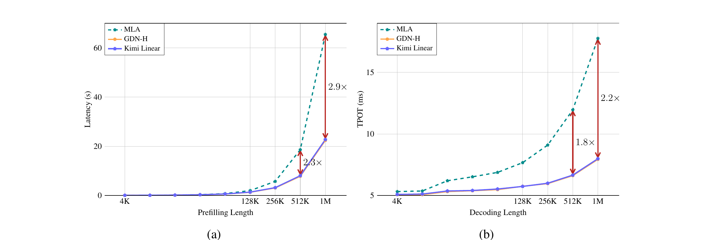
Source: Kimi Linear, Figure 7, page 13.
Figure 1(b)’s 6.3x result comes from a different serving condition. The smaller Kimi Linear cache permits a larger batch, producing 1.84 ms TPOT versus MLA’s 11.48 ms at 1M. This is a batching-capacity throughput result, not batch-one request latency. “Up to 75% KV-cache reduction” follows the 3:1 hybrid intuition: roughly three quarters of layers replace length-growing KV with fixed states, while MLA layers still cache tokens. Actual savings depend on KV dimension, recurrent state, convolution cache, dtype, and alignment.
A simple reporting rule avoids conflation. For “how long does one request take,” use the batch-one 2.2–2.3x result. For “how many requests can one device serve,” use up to 6.3x under the paper’s batching condition. For “how much cache memory is required,” use up to 75%. Every number needs its length, hardware, and batch condition.
10. Code cross-check: how the paper reaches FLA and Hugging Face
The current FLA KDA layer routes training and long prefill to a chunk kernel, while short inference sequences switch to a fused recurrent kernel below an implementation threshold. Projection paths fuse ShortConv, Swish, Q/K L2Norm, \(\beta\), and output gating to reduce intermediate memory traffic. The code also supports cumulative sequence lengths for variable batches, initial/final states, and context-parallel paths. These features are closer to a deployable operator contract than the paper pseudocode.
The Hugging Face configuration confirms 20 KDA and seven MLA layers among 27, with maximum position length 1,048,576. Implementation details should be pinned to a commit: FLA’s default chunk size, short-sequence threshold, gate layout, and state dtype can change. “Recurrent and chunkwise support” in a paper does not automatically cover continuous batching, prefix caching, quantization, tensor parallelism, and recovery; inference engines must integrate each feature.
FlashKDA pushes kernel optimization further with CUTLASS, chunk size 16, two main kernels, BF16 state storage, and FP32 FMA. The following figure summarizes the official H20 table. Across six workloads with \(T=8192,d=128\), it reports 1.85–2.31x over FLA KDA. These are operator latencies, not a complete Transformer layer.
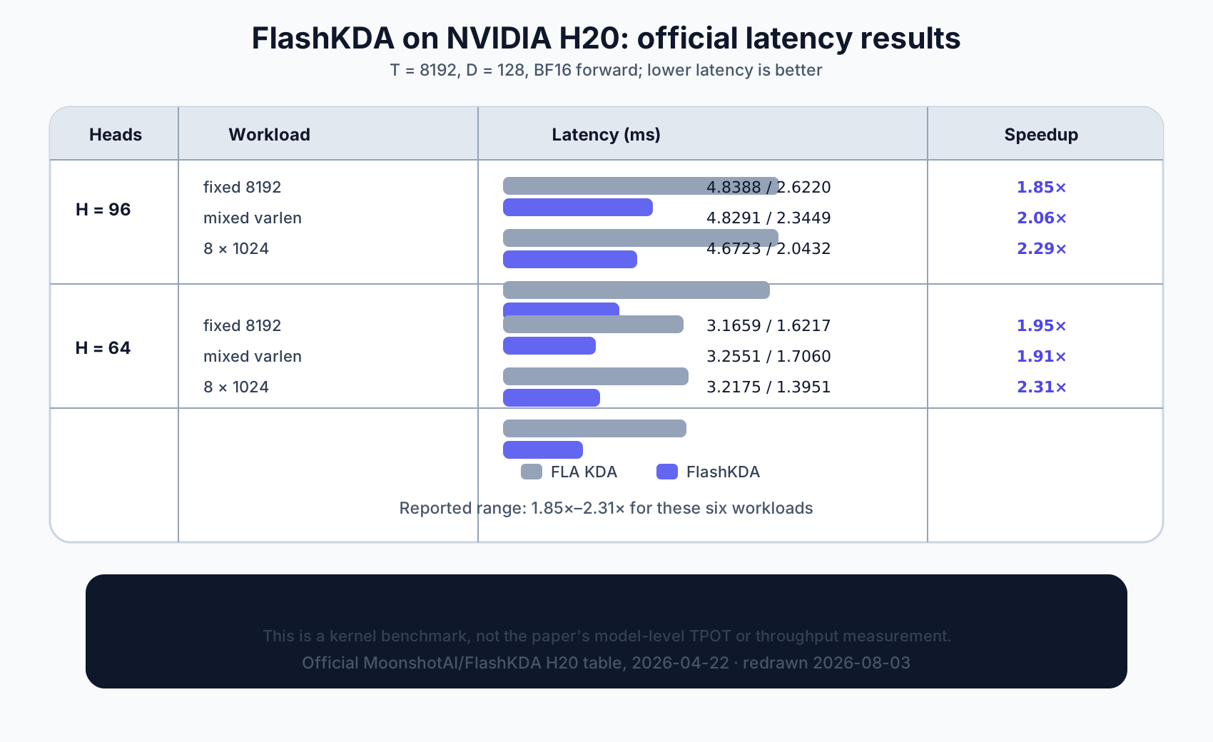
Data source: MoonshotAI/FlashKDA, official H20 benchmark dated 2026-04-22; accessed 2026-08-03.
This separation clarifies algorithmic complexity versus kernel constants. KDA versus MLA changes length-dependent work. Specialized WY/UT versus generic DPLR uses algebraic structure. FlashKDA versus FLA further improves tiling, state traffic, and instruction-level accumulation. The layers can compound, but no single context-free multiplier summarizes them.
11. KDA’s boundaries and three post-paper research lines
The first line decouples gates. Gated DeltaNet-2 identifies KDA’s shared scalar \(\beta_t\) for erase and write, then introduces channel-wise erase \(b_t\) and write \(w_t\):
\[ S_t = \left(I-k_t b_t^{\top}\right)\mathrm{Diag}(\alpha_t)S_{t-1} + k_t\left(w_t\odot v_t\right)^{\top}. \]
When \(b_t\) and \(w_t\) collapse to the same scalar control, the coupled KDA case is recovered. Finer gates increase expressivity but also projections, bandwidth, and optimization burden.
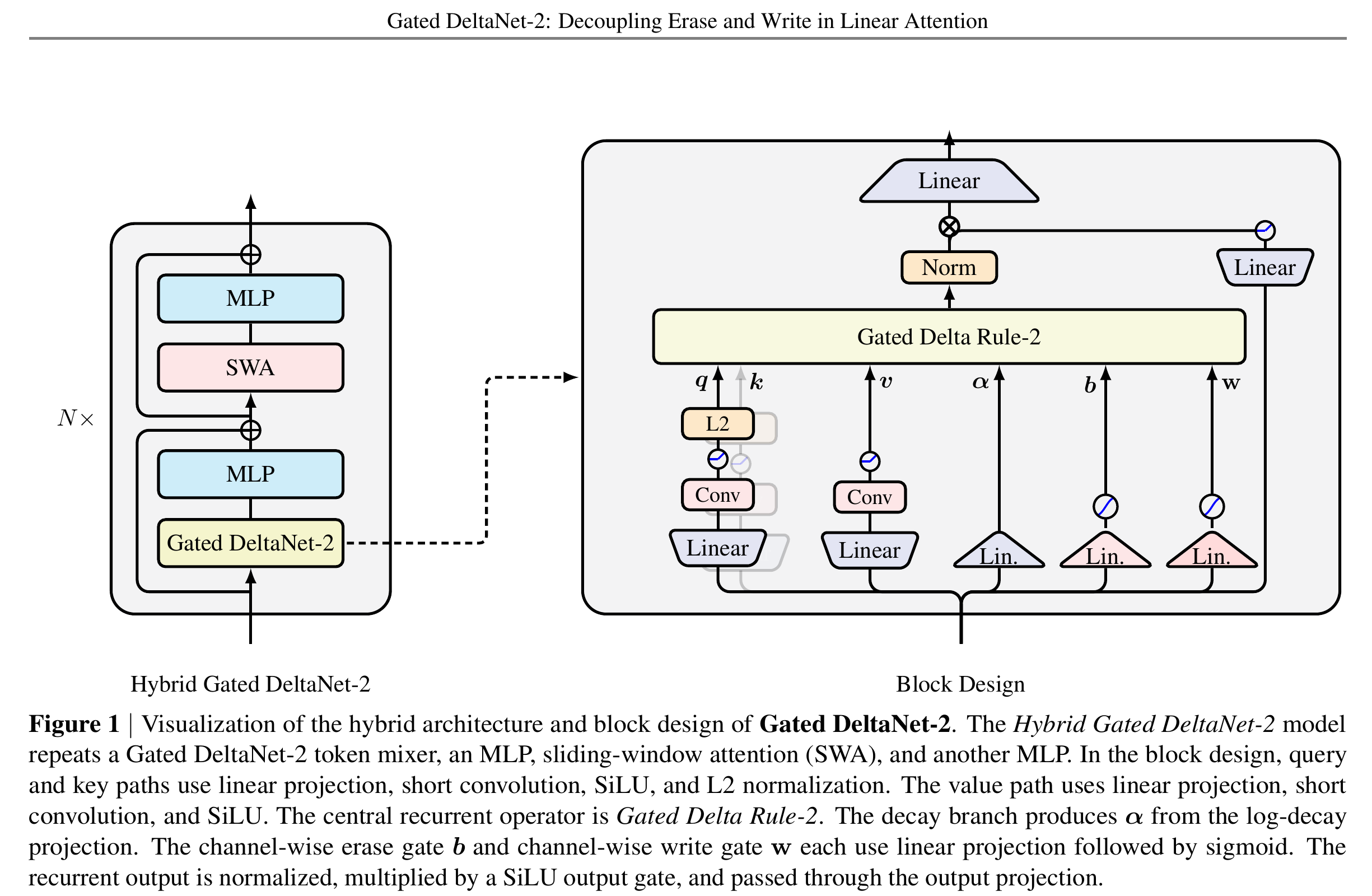
Source: Gated DeltaNet-2, Figure 1, page 6.
The second line is optimization. Preconditioned DeltaNet interprets state updates as online least squares. DeltaNet, Gated DeltaNet, and KDA behave like first-order descent on one-step loss without using regression curvature from key covariance. Highly correlated keys therefore make one scalar step size too fast in some directions and too slow in others. Approximate inverse-curvature preconditioning improves synthetic recall and 340M/1B language models. KDA improves forgetting coordinates; it does not solve the online regression condition number.
The third line is systems work. FlashKDA shows substantial room beyond the first efficient kernel, while adding reproducibility questions. Chunk 16 versus FLA’s chunk 64 changes parallelism and numerical association. BF16 state reduces traffic but may accumulate error over extreme lengths. Variable-length gains depend on the batch distribution. Future reports should include kernel microbenchmarks, full-layer time, complete-model prefill/decode, and serving throughput instead of selecting only the largest multiplier.
Four questions remain underexplored. How does effective fixed-state capacity scale with head count, \(d_k\), \(d_v\), and task entropy? Do channel-wise \(\alpha_t\) values learn interpretable time-scale specialization or merely flexible numerical compensation? Does 3:1 remain optimal for dense models, different MoE sparsity, and multimodal inputs? When does NoPE’s extrapolation benefit reverse on exact relative-position tasks? State probes, gate-distribution analysis, controlled capacity curves, and cross-scale ratio ablations could answer them.
12. Conclusion: KDA’s value is an executable structural constraint
Changing \(\alpha_t\) from a scalar to a vector looks minor, but it connects three levels. In modeling, different key channels can forget at different rates. In optimization, the delta rule preserves directed erase and write. In systems, the transition remains within a DPLR subclass that a specialized WY/UT algorithm can exploit. The 3:1 KDA/MLA hybrid acknowledges fixed-state capacity rather than claiming linear attention can replace token-level retrieval everywhere.
The strongest contribution is a coherent evidence chain rather than one maximum speedup. Synthetic tasks test learnability of finer forgetting; ablations select the hybrid ratio; scaling laws show about 1.16x compute at equal loss; long-context and RL results show that quality does not broadly collapse; kernel and systems measurements locate the deployment gains. Counterevidence is equally clear: LongBench V2 and Frames do not lead, batch-one TPOT is roughly 2.2x rather than 6.3x, and fixed-state compression still discards information.
My final view is that Kimi Linear is not a “Softmax killer.” It is a co-design of compressed memory, occasional exact retrieval, and executable GPU structure. The transferable lesson is not to copy one recurrence, but to choose a state edit expressive enough for the task and then verify that it can be chunked, fused, and tested stably. Subsequent work confirms that the design remains in motion: kernels can become faster, gates more independent, and updates curvature-aware. The real open question is not whether linear attention can run at one million tokens, but what a finite state retains on a given task—and what it forgets to get there.
References
- Moonshot AI. Kimi Linear: An Expressive, Efficient Attention Architecture, 2025.
- Moonshot AI. Kimi-Linear official repository.
- FLA contributors. Flash Linear Attention.
- Moonshot AI. FlashKDA, 2026.
- Yang et al. Gated DeltaNet: Improving Mamba2 with Delta Rule, 2024.
- Yang et al. Gated DeltaNet-2: Decoupling Erase and Write in Linear Attention, 2026.
- Preconditioned DeltaNet, 2026.
- Zhihu Kimi Linear reading, Scientific Spaces’ linear-attention history, MZeroMiko’s KDA derivation, and Zhiyuan Li’s affine derivation are explanatory comparisons only; technical claims are checked against the papers and code.