Entropy Collapse: Policy Entropy Consumption in LLM Reinforcement Learning
- Paper: The Entropy Mechanism of Reinforcement Learning for Reasoning Language Models
- Topic: Policy entropy consumption, performance saturation, and entropy control in LLM reinforcement learning
- Key result: RL consumes policy entropy rapidly at the beginning of training, and most performance gains also arrive in this early stage. If entropy then keeps decreasing monotonically, the model is more likely to settle into an overly deterministic local optimum.
In LLM reinforcement learning, entropy collapse refers to the rapid early drop of policy entropy followed by a continued drift toward nearly zero entropy. In practice, the model becomes overly confident: given similar states, it repeatedly selects a small set of high-probability tokens, response diversity shrinks, and the policy becomes easier to trap in a local optimum.
The pattern usually appears through two signals:
- Policy entropy decreases monotonically and eventually approaches zero.
- Validation performance reaches a plateau after an initial improvement.
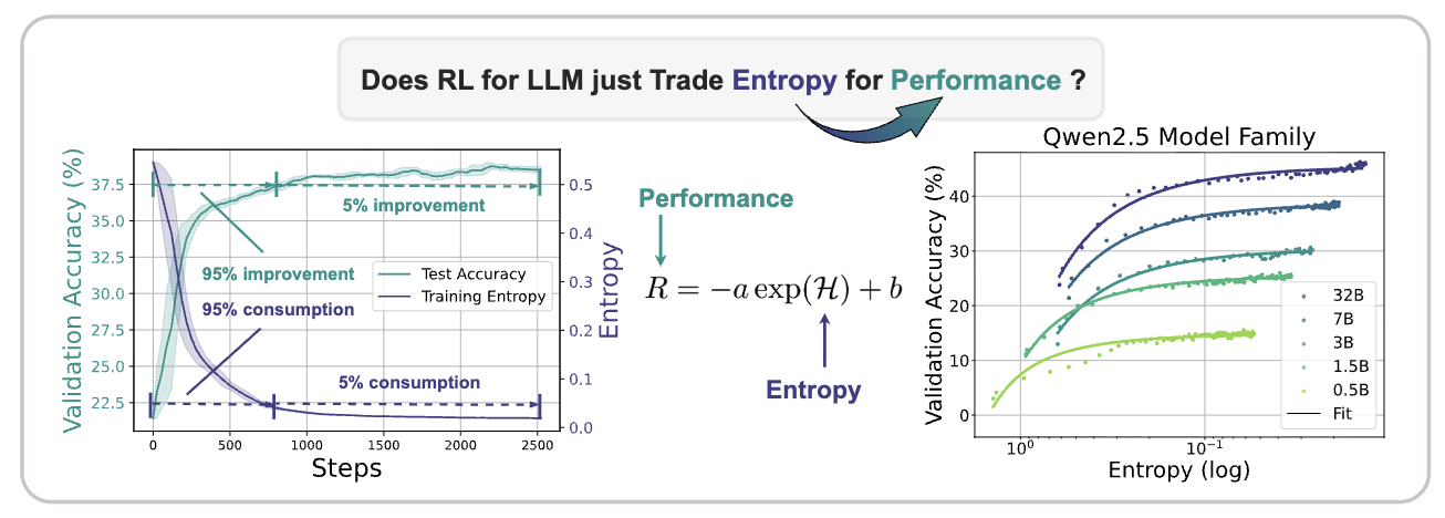
The Entropy Mechanism of Reinforcement Learning for Reasoning Language Models reports a direct empirical observation: during the first 200 RL training steps, the policy consumes 73% of its entropy while achieving 76% of its total performance gain. Training continues after that point, but entropy keeps falling while validation performance no longer improves at the same pace.
The paper also studies an empirical relationship between policy entropy and performance, measured by accuracy. For larger models, such as the 32B model in the figure, the coefficients \(a\) and \(b\) grow log-linearly with scale. This suggests that larger models convert entropy consumption into performance gains more efficiently, but they also reach the performance ceiling earlier. Lower entropy is not automatically better. In this setting, entropy behaves more like an exploration budget: once it is spent too early, later RL updates have little chance to discover new high-reward trajectories.
1. Definition of Policy Entropy
Policy entropy measures the randomness of a policy’s action choices. For language models, the policy is the LLM and an action is usually the next token. Given training data \(D\) and a policy \(\pi_\theta\), policy entropy can be written as:
\[ H(\pi_\theta, D) = -\mathbb{E}_{D,\pi_\theta}\left[\log \pi_\theta(y_t \mid y_{<t})\right] \]
In implementation, this quantity is usually averaged over generated tokens for each prompt in each batch of the training data \(D\).
Maximum-entropy RL uses entropy as a regularizer to balance exploration and exploitation. High entropy means that the policy still keeps several candidate actions alive. Low entropy means that probability mass has concentrated on a small number of actions. The latter is not always wrong, but if it happens too early, the policy can shrink before it has explored enough viable trajectories.
2. Why Entropy Collapse Restricts RL More Than SFT
Both SFT and RL can reduce token-level entropy, but they are affected in different ways. The main difference is that SFT has fixed supervised labels, while RL depends on trajectories sampled from the current policy.
SFT is supervised learning. It trains a model with parameters \(\theta\) so that its output distribution \(Q_0\) minimizes the training loss:
\[ C_{\text{SFT}}(\theta) = -\mathbb{E}_{(x,y)\sim P_{\text{data}}} \left[ \log Q_0(y|x) \right] \]
This objective follows empirical risk minimization: the dataset provides target answers, and the model increases the likelihood of those answers. SFT therefore tends to assign higher probability to supervised targets, reducing token-level policy entropy during one-step generation. Larger and better-trained models are often more certain, which partly explains why later RL stages can start from a low-entropy policy.
RL has a different dependency. The decoding process of the policy LLM \(\theta\) can be viewed as a stochastic policy distribution \(\pi(a|s)\), which induces a trajectory distribution \(q_\pi(\tau)\). Ideally, training would move toward a hypothetical optimal trajectory distribution \(P_{\text{opt}}(\tau)\). Unlike SFT, however, RL cannot sample directly from \(P_{\text{opt}}(\tau)\). It can only sample from the current policy’s \(q_\pi(\tau)\), score those samples, and update the policy from the observed rewards.
This is why entropy collapse is more damaging for RL. Once the current policy generates overly deterministic trajectories, the sampling space narrows quickly. A reward model or verifier can still score the sampled trajectories, but it cannot assign gradients to high-reward solutions that were never sampled. RL optimization does not stop completely; it becomes confined to the small region still covered by the low-entropy policy, and performance can easily plateau.
3. Methods for Mitigating Entropy Collapse
3.1 DAPO’s Clip-Higher Strategy
DAPO uses the following objective:
\[ \begin{aligned} \mathcal{J}_{\mathrm{DAPO}}(\theta) &= \mathbb{E}_{\substack{ (q,a)\sim D \\ \{o_i\}_{i=1}^{G}\sim \pi_{\theta_{\mathrm{old}}}(\cdot \mid q) }} \Bigg[ \frac{1}{\sum_{i=1}^{G}|o_i|} \sum_{i=1}^{G} \sum_{t=1}^{|o_i|} \min\left( r_{i,t}(\theta)\hat{A}_{i,t}, \bar{r}_{i,t}(\theta) \hat{A}_{i,t} \right) \Bigg] \end{aligned} \]
\[ \mathrm{s.t.}\quad 0 < \left| \left\{ o_i \mid \mathrm{is\_equivalent}(a,o_i) \right\} \right| < G \]
where
\[ r_{i,t}(\theta) = \frac{ \pi_{\theta}(o_{i,t}\mid q,o_{i,<t}) }{ \pi_{\theta_{\mathrm{old}}}(o_{i,t}\mid q,o_{i,<t}) } \]
\[ \hat{A}_{i,t} = \frac{ R_i-\mathrm{mean}\left(\{R_i\}_{i=1}^{G}\right) }{ \mathrm{std}\left(\{R_i\}_{i=1}^{G}\right) } \]
Here, \(\bar{r}_{i,t}(\theta)\) is the importance ratio after Clip-Higher clipping:
\[ \bar{r}_{i,t}(\theta) = \mathrm{clip} \left( r_{i,t}(\theta), 1-\varepsilon_{\mathrm{low}}, 1+\varepsilon_{\mathrm{high}} \right) \]
For comparison, GRPO uses symmetric clipping:
\[ \begin{aligned} \mathcal{J}_{\mathrm{GRPO}}(\theta) &= \mathbb{E}_{\substack{ (q,a)\sim D \\ \{o_i\}_{i=1}^{G}\sim \pi_{\theta_{\mathrm{old}}}(\cdot \mid q) }} \Bigg[ \frac{1}{G} \sum_{i=1}^{G} \frac{1}{|o_i|} \sum_{t=1}^{|o_i|} \left( \min\left( r_{i,t}(\theta)\hat{A}_{i,t}, \tilde{r}_{i,t}(\theta) \hat{A}_{i,t} \right) - \beta D_{\mathrm{KL}} \left( \pi_{\theta} \Vert \pi_{\mathrm{ref}} \right) \right) \Bigg] \end{aligned} \]
where
\[ r_{i,t}(\theta) = \frac{ \pi_{\theta}(o_{i,t}\mid q,o_{i,<t}) }{ \pi_{\theta_{\mathrm{old}}}(o_{i,t}\mid q,o_{i,<t}) } \]
\[ \tilde{r}_{i,t}(\theta) = \mathrm{clip} \left( r_{i,t}(\theta), 1-\varepsilon, 1+\varepsilon \right) \]
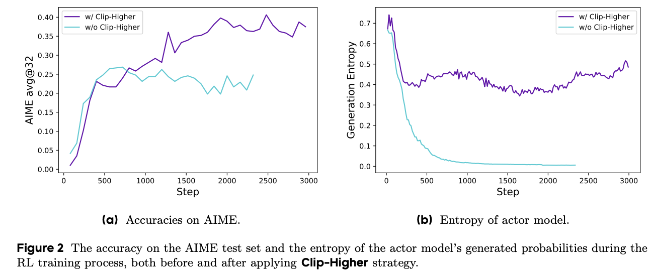
The effect of Clip-Higher can be understood through the probability ratio \(r_{i,t}(\theta)\) between the new and old policies for a given token. It relaxes the upper bound, allowing high-advantage tokens to receive larger probability increases, while keeping a lower-bound constraint to avoid unstable probability drops.
This asymmetric design targets a specific failure mode in entropy collapse. If low-probability but high-advantage tokens are clipped too aggressively by a symmetric bound, the policy is more likely to reinforce actions that are already high probability. Clip-Higher leaves more room for those tokens to rise, slowing down early policy contraction.
3.2 Covariance Regularization
The paper also analyzes how policy updates affect entropy and gives the following relationship:
\[ \Delta H \propto -\mathbb{E}_{s,a} \left[ \mathrm{Cov} \left( \log \pi_\theta(a \mid s), \Delta z_{s,a} \right) \right] \]
Here, \(\Delta z_{s,a}\) denotes the change in the logit.
In policy gradient, logit changes are proportional to action advantages, so the covariance term can be approximated as:
\[ \mathrm{Cov} \left( \log \pi_\theta(a \mid s), A(a) \right) \]
A high-covariance token is one for which \(\log \pi_\theta(a \mid s)\) and \(A(a)\) are strongly positively correlated. In other words, the token already has high probability and also receives high advantage. Further reinforcing such tokens pushes probability mass toward a small set of actions and accelerates the entropy drop.
Entropy control can therefore be framed as constraining gradient updates on high-covariance tokens. The paper discusses two variants.
Clip-Cov randomly clips gradients for some high-covariance tokens during policy-gradient updates. The clipping criterion uses a covariance threshold range:
\[ \omega_{\mathrm{low}} < \mathrm{Cov} < \omega_{\mathrm{high}} \]
The entropy level is controlled through the clipping ratio \(r\) and the threshold interval \((\omega_{\mathrm{low}}, \omega_{\mathrm{high}})\).
KL-Cov applies a KL penalty to the top-\(k\) tokens by covariance rank, and tunes entropy through the penalty coefficient \(\beta\):
\[ L_{\mathrm{policy}} = -\mathbb{E} \left[ \frac{\pi_\theta(y_i)}{\pi_{\mathrm{old}}(y_i)} A(y_i) \right] + \beta \cdot D_{\mathrm{KL}} \left( \pi_\theta \Vert \pi_{\mathrm{old}} \right)_{\mathrm{top}\text{-}k} \]
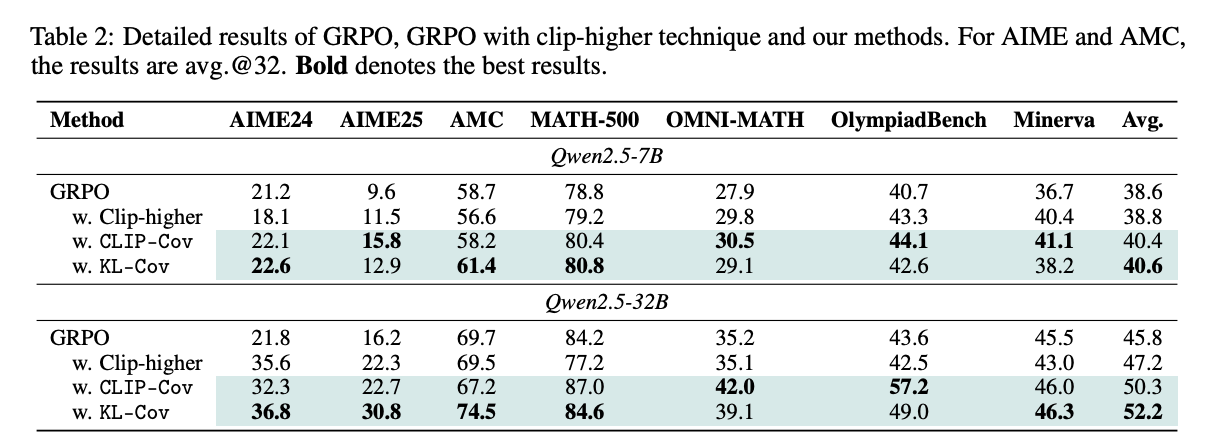
In the reported curves, KL-Cov produces a more stable entropy trajectory than Clip-Cov. This result is also intuitive: random clipping can prevent some high-covariance tokens from being further reinforced, but the KL penalty directly constrains their deviation from the old policy and gives a smoother control signal.
4. Summary
Entropy collapse is not merely a model becoming confident. It means that the exploration budget in RL is spent too early. SFT can tolerate low-entropy behavior because the supervised labels already provide the optimization direction. RL depends on trajectories sampled from the current policy; once policy entropy collapses, training can only optimize inside a narrow set of trajectories.
DAPO’s Clip-Higher strategy and covariance regularization address the same underlying issue: high-probability, high-advantage tokens should not monopolize early updates too quickly. Clip-Higher uses asymmetric clipping to leave room for low-probability high-advantage tokens. Covariance regularization identifies and constrains high-covariance tokens directly. Their shared goal is not to keep entropy high forever, but to make entropy decay more controlled so that performance gains are not exhausted too early.