PPO, DPO, and GRPO: Objectives and Training Loops for LLM Alignment
PPO, DPO, and GRPO are often presented as successive steps in one algorithmic progression, but they solve different optimization problems. PPO estimates advantages with a Critic and GAE. DPO rewrites KL-regularized preference learning as an offline classification loss. GRPO retains online policy optimization while replacing the Critic with group-relative rewards. This note compares the three methods through their objectives, preference or advantage signals, training loops, engineering costs, and practical boundaries.
1. PPO: Constrained Policy Optimization with a Value Baseline
1.1 Background and Motivation
Proximal Policy Optimization (PPO) was introduced by Schulman et al. in 2017. Its clipped surrogate objective approximates TRPO’s constraint on policy-update size with first-order optimization, reducing implementation cost while allowing several updates on the same rollout batch. In LLM alignment, PPO is commonly used in the reinforcement-learning stage of RLHF: a policy first undergoes SFT, a reward model learns from preference data, and PPO then optimizes that learned reward.
PPO’s central constraint is simple: improve reward without allowing the new policy to move too far from the sampling policy in one update.
1.2 PPO Objective
The objective makes the optimized quantity explicit:
\[ \mathcal{J}_{PPO}(\theta) = \mathbb{E}[q \sim P(Q), o \sim \pi_{\theta_{old}}(O|q)] \frac{1}{|o|} \sum_{t=1}^{|o|} \min \left[ \frac{\pi_\theta(o_t | q, o_{<t})}{\pi_{\theta_{old}}(o_t | q, o_{<t})} A_t, \text{clip}\left(\frac{\pi_\theta(o_t | q, o_{<t})}{\pi_{\theta_{old}}(o_t | q, o_{<t})}, 1-\varepsilon, 1+\varepsilon\right) A_t \right] \]
| Symbol | Meaning |
|---|---|
| \(q \sim P(Q)\) | A prompt sampled from the prompt distribution. |
| \(o \sim \pi_{\theta_{old}}(O \mid q)\) | A complete response sampled from the old policy. |
| \(\vert o\vert\) | Response length; averaging over tokens prevents longer responses from automatically receiving more loss weight. |
| \(\pi_\theta(o_t \mid q, o_{<t})\) | Probability assigned by the trainable policy to token \(o_t\). |
| \(\pi_{\theta_{\text{old}}}(o_t \mid q, o_{<t})\) | Corresponding probability under the sampling policy. |
| \(A_t\) | Token-level advantage, commonly estimated with GAE. |
| \(\varepsilon\) | PPO clipping threshold, often around \(0.1\) to \(0.2\). |
The objective multiplies each token’s advantage by the probability ratio between the new and old policies, then clips that ratio to limit the update.
Three components matter:
The importance ratio
\[ r_t(\theta) = \frac{\pi_\theta(o_t \mid q, o_{<t})}{\pi_{\theta_{old}}(o_t \mid q, o_{<t})} \]
measures how the policy probability changed.
The advantage \(A_t\) determines the direction and strength of the update. Positive advantages increase the action probability; negative advantages decrease it.
Clipping restricts \(r_t(\theta)\) to \([1-\varepsilon, 1+\varepsilon]\) in the surrogate objective, preventing a single batch from driving an excessive policy shift.
PPO and GRPO both use the importance ratio to adjust the gradient contribution of sampled tokens and clipping to limit update size.
1.3 Rollout Data and Advantage Estimation
1.3.1 Sampling Trajectories from the Old Policy
The old policy first samples a complete response:
\[ o = (o_1, \cdots, o_T) \sim \pi_{\theta_{old}}(O|q) \]
A reward model scores the response, and a KL penalty between the sampling policy and the reference policy contributes token-level rewards:
\[ r_{t}=r_{\varphi}(q,o_{\leq t})-\beta\log\frac{\pi_{\theta_{\text{old}}}(o_{t}|q,o_{<t})}{\pi_{\text{ref}}(o_{t}|q,o_{<t})} \]
The KL term discourages the policy from exploiting the reward model by moving too far from the reference model.
1.3.2 Estimating \(A_t\) with Reward, Value, and GAE
Reward alone does not say whether an action performed better than expected. PPO therefore uses the state-value function \(V(s_t)\) as a baseline:
- The Reward Model scores responses and supplies reward signals. It is frozen during the RL stage.
- The Critic predicts the expected return from the current state, \(V(s_t) = \mathbb{E}[G_t \mid s_t]\), and is trained alongside the Actor.
The state value represents the expected discounted return from the current state:
\[ V(s_t) \approx r_t + \gamma r_{t+1} + \gamma^2 r_{t+2} + \dots \]
Using the recursive approximation:
\[ V(s_t) \approx r_t + \gamma V(s_{t+1}) \]
PPO first computes the temporal-difference error:
\[ \delta_t = r_t + \gamma V(s_{t+1}) - V(s_t) \]
If \(\delta_t > 0\), the observed reward plus next-state value exceeded the Critic’s previous estimate.
GAE then accumulates current and future TD errors:
\[ \hat{A}_t = \delta_t + (\gamma \lambda)\delta_{t+1} + (\gamma \lambda)^2 \delta_{t+2} + \cdots + (\gamma \lambda)^{T-t} \delta_T \]
\(\lambda\) controls the bias-variance tradeoff. A common value is \(0.95\).
\[ \text{Advantage} = \text{weighted accumulation of (observed return - value expectation)} \]
1.3.3 Constructing the Return Target
The value target is:
\[ \text{Target}_t = V(s_t) + \hat{A}_t \]
Recall:
- \(\delta_t = r_t + \gamma V(s_{t+1}) - V(s_t)\)
- \(\hat{A}_t = \sum_{k=0}^{\infty} (\gamma \lambda)^k \delta_{t+k}\)
Expanding the target gives:
\[ \begin{aligned} \text{Target}_t &= \mathbf{V(s_t)} \\ &+ \underbrace{(r_t + \gamma V(s_{t+1}) - \mathbf{V(s_t)})}_{\delta_t} \\ &+ (\gamma\lambda) \underbrace{(r_{t+1} + \gamma V(s_{t+2}) - V(s_{t+1}))}_{\delta_{t+1}} \\ &+ (\gamma\lambda)^2 \delta_{t+2} + \dots \end{aligned} \]
After canceling \(V(s_t)\):
\[ \text{Target}_t = r_t + \gamma V(s_{t+1}) + (\gamma\lambda)(r_{t+1} + \gamma V(s_{t+2}) - V(s_{t+1})) + \dots \]
The two terms containing \(V(s_{t+1})\) become:
\[ \gamma V(s_{t+1}) - \gamma\lambda V(s_{t+1}) = \gamma (1-\lambda) V(s_{t+1}) \]
Continuing the expansion:
\[ \begin{aligned} \text{Target}_t &= r_t + \gamma (1-\lambda)V_{t+1} \\ &+ \gamma\lambda r_{t+1} + (\gamma\lambda) \gamma (1-\lambda)V_{t+2} \\ &+ (\gamma\lambda)^2 \left[ r_{t+2} + \gamma (1-\lambda)V_{t+3} + \dots \right] \end{aligned} \]
The general form is:
\[ G_t^\lambda = (1-\lambda) \sum_{n=1}^{\infty} \lambda^{n-1} G_t^{(n)} \]
where \(G_t^{(n)}\) is an n-step return:
- \(G_t^{(1)} = r_t + \gamma V(s_{t+1})\)
- \(G_t^{(2)} = r_t + \gamma r_{t+1} + \gamma^2 V(s_{t+2})\)
- \(G_t^{(\infty)} = G_t\), the Monte Carlo return
The target built from \(V_{old} + A\) is therefore a weighted average of n-step returns. Larger \(\lambda\) values rely more on long-horizon observed rewards; smaller values rely more on short-horizon bootstrapping.
If \(\lambda = 1\), the target reduces to the Monte Carlo return. If \(\lambda < 1\), it becomes a lower-variance approximation that still uses the Critic to smooth sampled returns.
The estimation chain is:
\[ \text{RM score} \xrightarrow{r_t} \text{combine with Critic } V(s_t) \xrightarrow{\text{GAE}} \hat{A}_t \]
The Critic directly affects the signal-to-noise ratio of the advantage estimate. A biased Critic can therefore degrade the Actor update.
1.4 Training the Critic
In typical LLM-RLHF implementations, the Critic is initialized from Actor or Reward Model weights and adds a value head that maps hidden states to scalars. Actor and Critic may share parameters or run as separate models. At each step, the Critic predicts \(V(s_t)\) and regresses toward an estimated return target:
\[ \min_{V} \mathbb{E}_{s_t, R} \left[ (V(s_t) - R)^2 \right] \]
For a fixed state, let the prediction be \(v\) and the future return be the random variable \(R\):
\[ \min_{v} \mathbb{E}[(v - R)^2] \]
Differentiating with respect to \(v\):
\[ \frac{d}{dv} \mathbb{E}[(v - R)^2] = 2\mathbb{E}[v - R] = 0 \]
Thus:
\[ V(s_t) = \mathbb{E}[R \mid s_t] \]
\(V(s_t)\) is a conditional expectation and a predictive baseline, not an attempt to reproduce one sampled reward trajectory exactly.
1.5 PPO Training Loop
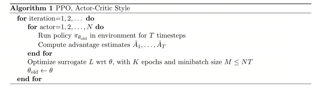
One PPO rollout-update cycle has three stages.
Stage 1: Rollout and scoring
- The old Actor generates responses and records states, actions, and rewards.
- The old Critic predicts \(V_{old}(s)\) for the sampled states.
Stage 2: Advantage and return-target computation
The networks remain fixed while the rollout batch is converted into:
- \(\hat{A}\) from rewards and \(V_{old}\) through GAE.
- \(\text{Returns} = V_{old} + \hat{A}\).
These tensors are detached from the computation graph and remain fixed during the following update epochs.
Stage 3: Optimization
- The Actor minimizes the clipped policy loss using \(\hat{A}\).
- The Critic minimizes a value-regression loss using \(\text{Returns}\).
PPO is an on-policy policy-optimization method, but it uses importance ratios and clipping to reuse a near-on-policy batch for a limited number of updates. Recomputing and backpropagating through the advantage after every Critic update would make the surrogate target drift during optimization.
2. DPO: Rewriting Preference Learning as a Classification Loss
2.1 Core Idea and Derivation
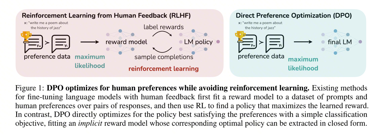
PPO requires an explicit Reward Model, online rollouts, advantage estimation, and Critic updates. Direct Preference Optimization (DPO), introduced by Rafailov et al. in 2023, asks whether a policy can instead learn directly from preference pairs.
DPO uses the relationship between a KL-regularized RLHF optimum and the log-probability ratio between the policy and reference model. The derivation has two steps:
- Derive the closed-form optimal policy under a KL-regularized reward objective.
- Substitute that expression into the Bradley-Terry preference model to obtain a classification loss over preference pairs.
2.1.1 From KL-Regularized Optimization to a Closed-Form Policy
The RLHF objective maximizes expected reward while penalizing divergence from the reference policy:
\[ \max_{\pi_\theta} \; \mathbb{E}_{x \sim \mathcal{D},\, y \sim \pi_\theta(\cdot|x)} \left[ r(x, y) \right] - \beta \, \text{KL}\!\left[\pi_\theta(\cdot|x) \;\Vert \; \pi_{\text{ref}}(\cdot|x)\right] \]
Its optimal policy has the form:
\[ \pi^*(y|x) = \frac{1}{Z(x)} \, \pi_{\text{ref}}(y|x) \, \exp\!\left(\frac{r(x,y)}{\beta}\right) \]
where:
\[ Z(x) = \sum_y \pi_{\text{ref}}(y \mid x) \exp\!\left(\frac{r(x,y)}{\beta}\right) \]
The optimum exponentially reweights the reference policy according to reward. Larger \(\beta\) values make the reweighting more conservative.
2.1.2 Solving for the Implicit Reward
Taking logs and rearranging:
\[ r(x, y) = \beta \log \frac{\pi^*(y|x)}{\pi_{\text{ref}}(y|x)} + \beta \log Z(x) \]
The reward can therefore be represented by a policy-reference log ratio plus a prompt-dependent constant.
2.1.3 Substituting into the Bradley-Terry Model
For a preferred response \(y_w\) and rejected response \(y_l\):
\[ p(y_w \succ y_l | x) = \sigma\!\left(r(x, y_w) - r(x, y_l)\right) \]
Substituting the implicit reward yields:
\[ p(y_w \succ y_l | x) = \sigma\!\left(\beta \log \frac{\pi^*(y_w|x)}{\pi_{\text{ref}}(y_w|x)} - \beta \log \frac{\pi^*(y_l|x)}{\pi_{\text{ref}}(y_l|x)}\right) \]
The prompt-only term \(\beta \log Z(x)\) cancels in the reward difference. DPO can therefore train the policy directly on preference pairs without explicitly estimating \(Z(x)\) or training a separate Reward Model.
2.2 DPO Loss
Taking the negative log-likelihood of the preference probability gives:
\[ \mathcal{L}_{\text{DPO}}(\theta) = -\mathbb{E}_{(x, y_w, y_l) \sim \mathcal{D}} \left[ \log \sigma\!\left( \beta \log \frac{\pi_\theta(y_w|x)}{\pi_{\text{ref}}(y_w|x)} - \beta \log \frac{\pi_\theta(y_l|x)}{\pi_{\text{ref}}(y_l|x)} \right) \right] \]
Define the implicit reward:
\[ \hat{r}_\theta(x, y) = \beta \log \frac{\pi_\theta(y \mid x)}{\pi_{\text{ref}}(y \mid x)} \]
Then:
\[ \mathcal{L}_{\text{DPO}} = -\mathbb{E}\left[\log \sigma\!\left(\hat{r}_\theta(x, y_w) - \hat{r}_\theta(x, y_l)\right)\right] \]
The optimization increases the implicit-reward margin between chosen and rejected responses.
The gradient is:
\[ \nabla_\theta \mathcal{L}_{\text{DPO}} = -\beta \, \mathbb{E}\!\left[\underbrace{\sigma\!\left(\hat{r}_\theta(x, y_l) - \hat{r}_\theta(x, y_w)\right)}_{\text{implicit weight}} \left[\nabla_\theta \log \pi_\theta(y_w|x) - \nabla_\theta \log \pi_\theta(y_l|x)\right]\right] \]
Preference pairs that the policy already ranks correctly receive smaller weights; incorrectly ranked pairs receive larger corrections.
The loss requires policy and reference-model log probabilities for both chosen and rejected responses. It does not require Reward Model scoring, a Critic, or GAE, so its training pipeline is close to supervised fine-tuning.
2.3 The Constraining Roles of the Reference Policy and \(\beta\)
DPO has no per-sample explicit KL penalty in its practical loss. KL regularization appears at the start of the theoretical derivation and influences the loss through the reference policy and \(\beta\), but the trained policy is not guaranteed to satisfy a fixed KL limit.
2.3.1 Log-Probability Ratios Define the Implicit Reward
The log ratio measures how much the policy raises or lowers the probability of a response relative to the reference model. DPO optimizes the difference:
\[ \hat{r}_\theta(x, y_w) - \hat{r}_\theta(x, y_l) \]
When the policy already gives the chosen response a higher relative probability, the sigmoid weight decreases. When the ranking is wrong, the gradient grows. Because the loss focuses on a difference between two responses rather than absolute policy-reference KL, training should still monitor KL, response length, and generation quality.
2.3.2 Theoretical Source and Practical Boundary
The reference policy and \(\beta\) enter DPO through the KL-regularized RLHF objective:
- \(\beta\) scales the chosen-rejected relative log-ratio margin and changes optimization strength.
- \(\pi_{\text{ref}}\) anchors the objective to preference changes relative to the initial policy.
DPO’s derivation includes KL regularization, but its practical loss is not equivalent to applying an explicit KL penalty at every step. Neither \(\beta\) nor the reference model replaces empirical monitoring.
2.4 DPO Compared with PPO
| Dimension | PPO | DPO | Practical effect |
|---|---|---|---|
| Training pipeline | SFT → Reward Model → online PPO | SFT → offline preference optimization | DPO removes independent RM training and online rollouts. |
| Reward signal | An independent RM scores generated responses | Policy-reference log ratios define implicit rewards | DPO avoids separately training an RM but can still overfit preference data. |
| Optimization | Actor-Critic, GAE, clipping | Classification loss over chosen/rejected pairs | DPO is closer to supervised learning and needs no value estimator. |
| Sampling during training | Continuously samples from the current policy | Uses static offline preference pairs | DPO is cheaper to train but cannot actively explore new responses. |
| Model state | Actor, Critic, RM, Reference | Policy, Reference | DPO simplifies memory and distributed-state management. |
| Main hyperparameters | Actor/Critic learning rates, \(\gamma\), \(\lambda\), \(\varepsilon\), KL coefficient, and others | Learning rate, \(\beta\), and others | DPO has fewer moving parts, but \(\beta\), data quality, and length bias remain important. |
DPO depends on the quality and coverage of offline preference data and cannot continuously explore response space like PPO. Online DPO and IPO address different parts of this limitation.
GRPO simplifies PPO from another direction: it retains online RL but removes the Critic, estimating advantages from normalized group rewards.
3. GRPO: Replacing the Critic with Group-Relative Rewards
3.1 Background and Motivation
PPO and DPO represent two different training paths:
- PPO keeps the full online RL pipeline with RM scoring, Critic estimation, GAE, importance ratios, and clipping.
- DPO optimizes offline preference pairs without an online RL loop.
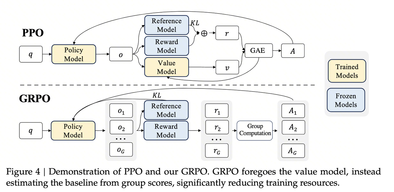
Group Relative Policy Optimization (GRPO), introduced in the 2024 DeepSeekMath paper, retains online sampling while removing the Critic:
It replaces the Critic’s value estimate with relative rewards among multiple responses to the same prompt.
This changes both resource requirements and error sources:
- It removes Critic parameters, gradients, optimizer states, and distributed communication. The actual savings depend on how the Actor, Reference, and Reward Model are deployed.
- It removes Critic training and the instability caused by value-estimation error.
The remaining question is how to construct \(\hat{A}_{i,t}\) without a learned value baseline.
3.2 Advantage Estimation from Group Comparisons
For one prompt \(q\), GRPO samples \(G\) complete responses \(o_1, o_2, \dots, o_G\) from \(\pi_{\theta_{\text{old}}}\). It then constructs advantages according to the granularity of the reward signal.
3.2.1 Outcome Supervision: One Advantage per Sequence
An outcome reward model assigns scalar rewards \(r_1, r_2, \dots, r_G\). GRPO normalizes them within the group:
\[ \tilde{r}_i = \frac{r_i - \text{mean}(\mathbf{r})}{\text{std}(\mathbf{r})} \]
\(\tilde{r}_i > 0\) means the response performed above the group mean; \(\tilde{r}_i < 0\) means it performed below the mean.
The normalized outcome reward is broadcast to every token in the response:
\[ \hat{A}_{i,t} = \tilde{r}_i \quad (\text{for every position } t \text{ in response } i) \]
This is a coarse credit-assignment approximation. It works with final-answer rewards but cannot identify which reasoning step was useful or incorrect.
3.2.2 Process Supervision: Accumulated Step-Level Advantages
With a Process Reward Model, step rewards are normalized:
\[ \tilde{r}_{i,j} = \frac{r_{i,j} - \text{mean}(\text{GroupRewards})}{\text{std}(\text{GroupRewards})} \]
For a token \(t\) belonging to reasoning step \(j\), GRPO accumulates future normalized step rewards:
\[ \hat{A}_{i,t} = \sum_{k=j}^{K_i} \tilde{r}_{i,k} \quad (\text{where token } t \text{ belongs to step } j) \]
Earlier steps receive credit or blame for their effect on subsequent reasoning. Under either outcome or process supervision, group statistics replace the Critic: the group mean approximates a baseline and the standard deviation normalizes scale.
3.3 GRPO Objective
GRPO retains PPO’s importance ratio and clipping while averaging across a response group:
\[ \mathcal{J}_{GRPO}(\theta) = \mathbb{E}[q \sim P(Q), \{o_i\}_{i=1}^{G} \sim \pi_{\theta_{old}}(O|q)] \frac{1}{G} \sum_{i=1}^{G} \frac{1}{|o_i|} \sum_{t=1}^{|o_i|} \left\{ \min \left[ \rho_{i,t} \hat{A}_{i,t}, \; \text{clip}(\rho_{i,t}, 1-\varepsilon, 1+\varepsilon) \hat{A}_{i,t} \right] - \beta \, \text{KL}[\pi_\theta \Vert \pi_{\text{ref}}] \right\} \]
where:
\[ \rho_{i,t} = \frac{\pi_\theta(o_{i,t} \mid q, o_{i,<t})}{\pi_{\theta_{old}}(o_{i,t} \mid q, o_{i,<t})} \]
3.3.1 Group Sampling and Two-Level Averaging
GRPO adds an outer average over the \(G\) sampled responses:
- \(\frac{1}{G}\sum_{i=1}^{G}\) averages across responses to the same prompt.
- \(\frac{1}{\vert o_i \vert}\sum_{t=1}^{\vert o_i \vert}\) averages across tokens within one response.
Group sampling is required to estimate relative advantages and can also reduce gradient variance through multi-sample averaging.
3.3.2 A Different Advantage Source
| Dimension | PPO | GRPO |
|---|---|---|
| Advantage source | Critic \(V(s_t)\) + GAE | Normalized group rewards |
| Additional value model | Critic | None |
| Granularity | Token-level through TD errors | Sequence-level for outcome rewards; step-level for process rewards |
Responses above the group mean receive positive advantages and higher generation probabilities; responses below the mean receive negative advantages and lower probabilities.
3.4 GRPO Training Loop
3.4.1 Three Nested Loops
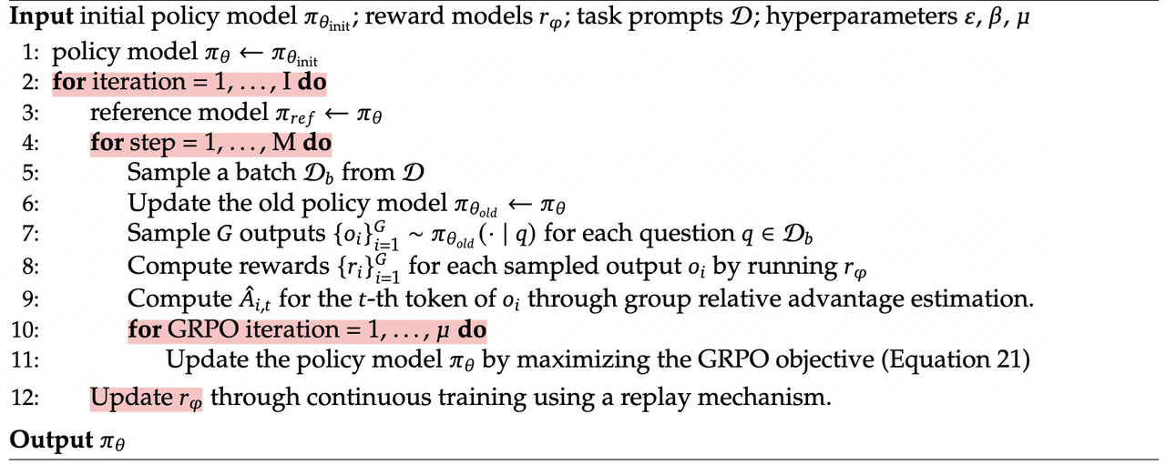
GRPO training uses three nested loops.
Outer iteration loop
- Refresh the reference policy from the current policy, then freeze it for the iteration.
- Optionally update the Reward Model as the policy distribution changes.
Sampling step loop
- Sample a prompt batch \(\mathcal{D}_b\).
- Snapshot the current policy as \(\pi_{\theta_{\text{old}}}\).
- Generate \(G\) responses per prompt.
- Score the responses and compute \(\hat{A}_{i,t}\).
- Store prompts, responses, advantages, and old-policy probabilities.
GRPO update loop
Reuse the fixed rollout batch for \(\mu\) optimization epochs, split into mini-batches, and optimize the GRPO objective.
The loops separately control reference-policy refresh frequency, rollout cadence, and data-reuse count.
3.4.2 Why the Importance Ratio Is Necessary
Rollouts come from \(\pi_{\theta_{\text{old}}}\), but \(\pi_\theta\) changes after every gradient update. The ratio corrects for this distribution mismatch:
| Ratio | Meaning | Training effect |
|---|---|---|
| \(\rho > 1\) | The new policy assigns the token higher probability | Amplifies a positively advantaged action before clipping |
| \(\rho < 1\) | The new policy assigns the token lower probability | Reduces the sampled action’s contribution |
| \(\rho \approx 1\) | New and old policies agree | Little correction |
Clipping limits \(\rho_{i,t}\) to the effective range around \([1-\varepsilon, 1+\varepsilon]\) in the surrogate objective. The ratio corrects for the gap between current and sampling policies; clipping limits update size. Together they support limited reuse of each rollout batch.
3.5 Comparison Summary
| Dimension | PPO | DPO | GRPO |
|---|---|---|---|
| Training method | Online Actor-Critic RL | Offline preference optimization | Online group-relative RL |
| Reward or preference signal | Explicit RM reward + Critic baseline | Chosen/rejected preference pairs | Explicit or verifiable rewards + group baseline |
| Advantage estimation | Critic + GAE | No policy-gradient advantage | Group reward normalization |
| Online sampling | Required | Not required by standard DPO | Required, with \(G\) responses per prompt |
| Main model components | Actor, Critic, RM, Reference | Policy, Reference | Actor, reward function or RM, Reference |
| Main risks | RM bias, Critic bias, complex training pipeline | Preference coverage, length bias, out-of-distribution generalization | Group reward variance, sparse rewards, coarse sequence-level credit assignment |
| Suitable settings | RLHF requiring online exploration and fine-grained value estimation | Offline preference data with an emphasis on training efficiency | Reasoning tasks with reliable verifiable rewards, such as mathematics and code |
| Representative work | InstructGPT | DPO, Zephyr, Tulu 2 | DeepSeekMath, DeepSeek-R1 |
4. Further Reading
Original and primary papers
- Proximal Policy Optimization Algorithms (Schulman et al., 2017) — Introduces PPO’s clipped surrogate objective and compares it with TRPO and related methods.
- Training language models to follow instructions with human feedback (Ouyang et al., 2022) — Describes the SFT → RM → PPO training pipeline used for InstructGPT.
- Direct Preference Optimization: Your Language Model is Secretly a Reward Model (Rafailov et al., 2023) — Derives the preference-classification loss from a KL-regularized optimal policy.
- DeepSeekMath: Pushing the Limits of Mathematical Reasoning in Open Language Models (Shao et al., 2024) — Introduces GRPO and evaluates group-relative optimization for mathematical reasoning.
- DeepSeek-R1: Incentivizing Reasoning Capability in LLMs via Reinforcement Learning (DeepSeek-AI, 2025) — Documents the use of GRPO in large-scale reasoning-model training.
Additional reading
- A General Theoretical Paradigm to Understand Learning from Human Feedback (Azar et al., 2023) — Introduces IPO and analyzes preference optimization under finite data.
- Self-Play Fine-Tuning Converts Weak Language Models to Strong Language Models (Chen et al., 2024) — Explores preference learning through self-play.
- RLHF Workflow: From Reward Modeling to Online RLHF (Dong et al., 2024) — Studies engineering workflows from offline preference optimization to online RLHF.
- Is DPO Superior to PPO for LLM Alignment? A Comprehensive Study (Xu et al., 2024) — Compares PPO and DPO across multiple alignment settings.